Beyond LoRA: Is Sparsity-Induced Adaptation Better?

Abstract

Low-rank adaptation (LoRA) and its variants provide a memory- and compute-efficient alternative to full fine-tuning of pre-trained models. However, questions remain about the comparative generalizability of these approaches and how the structural restrictions on low-rank updates preserve effective adaptation performance. We present a historical framing, covering the past (full fine-tuning and original LoRA), the present (different variants of LoRA), and propose simpler, cheaper, parameter-efficient extensions by inducing sparsity within existing LoRA variants: Cheap LoRA (cLA), training a single low-rank factor with the other fixed (deterministically or, in its randomized variant, stochastically), and the chained circulant variant, c³LA.

We frame cLA as a structured instance of asymmetric LoRA, serving as a controlled column-subspace restriction of full fine-tuning. We derive information-theoretic generalization error bounds for these variants, marking one of the first endeavors in this area. Empirically, we evaluate 11 fine-tuning methods across 10 pre-trained models and 14 datasets, analyzing the fine-tuned models' performance and generalization using tools such as loss landscapes and spectral analysis. Despite the sensitivity of fine-tuned models to the pre-trained model, datasets, and other factors, our study suggests that restricting LoRA-based PEFT methods' adaptation to a sparse, structured column space remains competitive across tasks with their parameter-matched baselines while reducing up to 10% training time and peak GPU memory up to 15%, even with a naïve, non-optimized, sparse implementation. Our theoretical and empirical generalization measures provide a more consistent and principled approach to their cost-effective adaptation than commonly used analytical tools.

Motivation: Parameter Count vs. Parameter Geometry

PEFT methods are often compared by trainable parameter count, but parameter count alone does not explain how an update changes the pretrained model. Two adapters can have nearly identical parameter budgets while occupying very different subspaces of the original weight matrix, producing different performance, robustness, and generalization behavior.

Our central question is therefore geometric: which structured restrictions on low-rank updates preserve useful adaptation, and how far can we restrict the column space before the model stops adapting well? By inducing structured sparsity into LoRA-style updates, cLA and its chained/randomized variants provide a controlled way to study whether the location and structure of the update matters as much as, or more than, the number of trainable parameters while leveraging the sparse structure to save runtime and memory.

Key Contributions

Overview of Proposed Sparsity-induced LoRA variants

Algorithms

The pseudocode below sketches the sparse adaptation mechanisms used by the proposed variants.

Given pretrained layer W0 ∈ R^{n×m}
Choose rank r and scale α

Set A = [ I_r | 0_{r×(m-r)} ]
Initialize B = 0_{n×r}

For each training step:
  Compute loss L using W = W0 + (α/r) · B · A
  Update B ← B − η · ∇_B L

Return adapted layer W

Given pretrained layer W0 ∈ R^{n×m}
Choose rank r, chain length k, scale α

For j = 1..k:
  Define A_j as a shifted selector
    A_1 = [ I_r | 0 | 0 | ... ]
    A_2 = [ 0 | I_r | 0 | ... ]
    ...
  Initialize B_j = 0_{n×r}

For j = 1..k:
  For each training step:
    Compute loss L using
      W = W0 + Σ_{t=1..j} (α/r) · B_t · A_t
    Update B_j ← B_j − η · ∇_{B_j} L

Return adapted layer W

Given pretrained layer W0 ∈ R^{n×m}
Choose rank r and scale α

Sample a fixed randomized selector A
Initialize B = 0_{n×r}

For each training step:
  Compute loss L using W = W0 + (α/r) · B · A
  Update B ← B − η · ∇_B L

Return adapted layer W

Given pretrained layer W0 ∈ R^{n×m}
Choose rank r, chain length k, scale α

For j = 1..k:
  Sample a fixed randomized selector without replacement A_j from the shifted selectors of c^{3}LA
  Initialize B_j = 0_{n×r}

For j = 1..k:
  For each training step:
    Compute loss L using
      W = W0 + Σ_{t=1..j} (α/r) · B_t · A_t
    Update B_j ← B_j − η · ∇_{B_j} L

Return adapted layer W

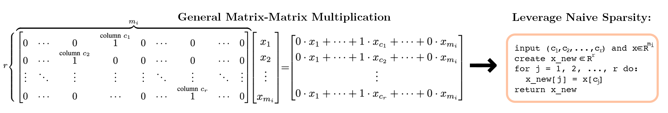
Naïve sparse implementation

The sparse construction can be implemented without multiplying by the full fixed selector. For cLA and random-cLA, the selector A simply chooses r coordinates of the input. Instead of computing A(x) as a dense matrix multiplication, the implementation stores the selected column indices and directly gathers [x_c1, …, x_cr]. This avoids unnecessary selector FLOPs and helps explain the observed runtime and memory reductions.

Sparse LoRA variants can exploit the fact that the fixed selector only gathers a small set of input columns.

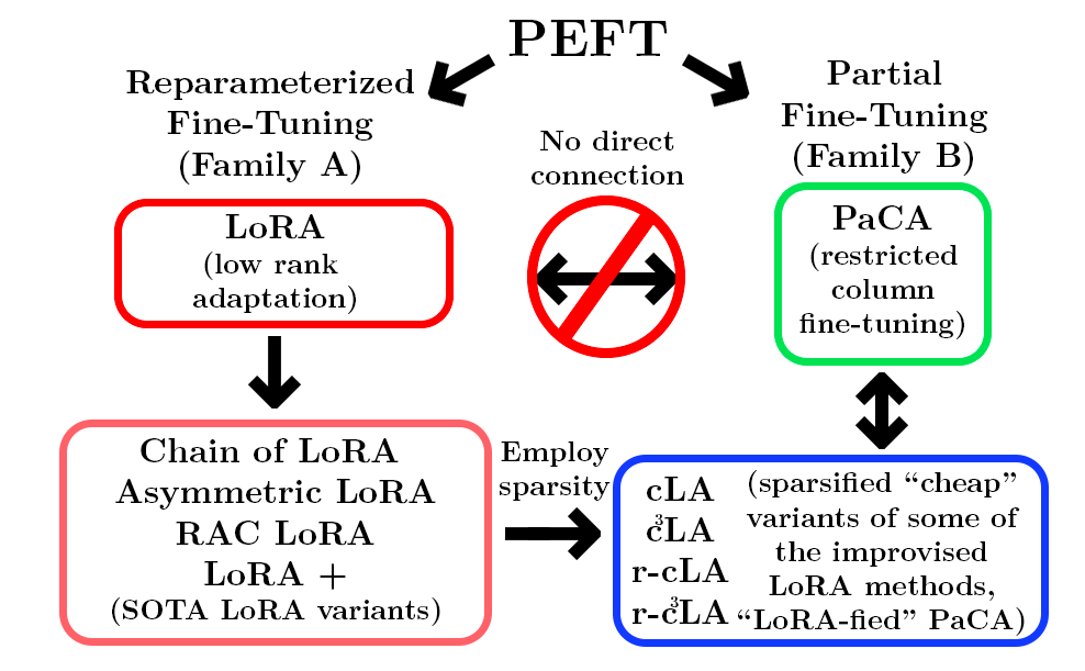
Bridge to PaCA

Partial Connection Adaptation (PaCA) was motivated from a systems perspective: it reduces activation memory by only training a subset of the columns of each original layers' weights. Our sparse LoRA variants provide a theoretical bridge between PaCA and LoRA; when PaCA fine-tunes the first r columns of the pretrained layer, it updates the same parameters as cLA, thus PaCA can be reframed theoretically as a LoRA style update using cLA with a corresponding selector matrix A, allowing us to apply theoretical results from LoRA to PaCA. This does not imply that PaCA is strictly better than the cLA variants, since there are many benefits of the LoRA structure (being able to switch between multiple tasks easily, for example) that PaCA does not retain.

Sparsity-induced LoRA variants connect reparameterized fine-tuning and partial fine-tuning.

Theoretical Generalization Bounds of LoRA variants

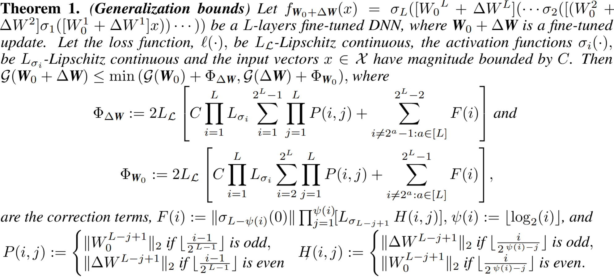
Theorem 1 is a general bound for an arbitrary fully connected L-layer neural network. It upper bounds the generalization error of the fine-tuned model W₀ + ΔW using the generalization behavior of either the pretrained backbone or the update. This makes it a reusable template: once a PEFT method specifies the structure of ΔW, the theorem can comment on its generalizability.

The standalone correction terms Φ_ΔW and Φ_W0 collect the Lipschitz constants of the loss and activations, layerwise spectral norms of the base and update weights, and zero-activation offset terms from recursively collapsing the difference between the fine-tuned and pretrained networks.

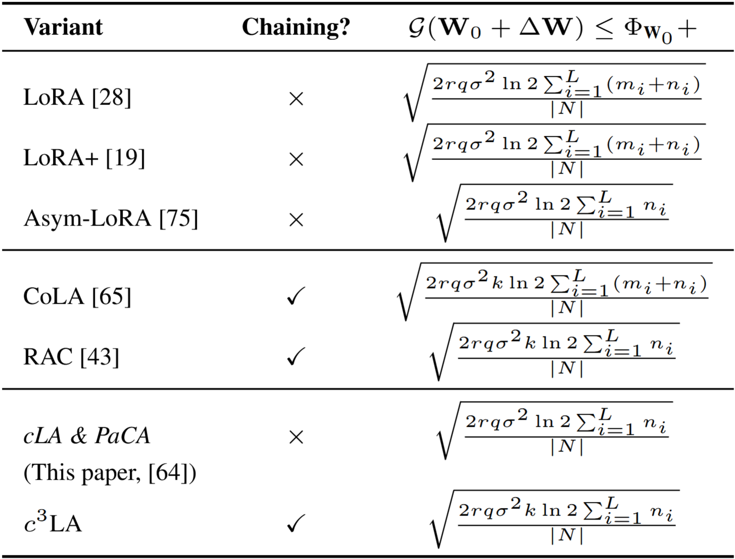
With the additional assumption that the loss function ℓ(·) is σ-sub-Gaussian, we obtain upper bounds for the LoRA variants studied in this paper and for PaCA. The table below summarizes these bounds. For the derivation of each variant-specific bound, see Appendix D.1.6 of the paper.

Benchmarking and Evaluation

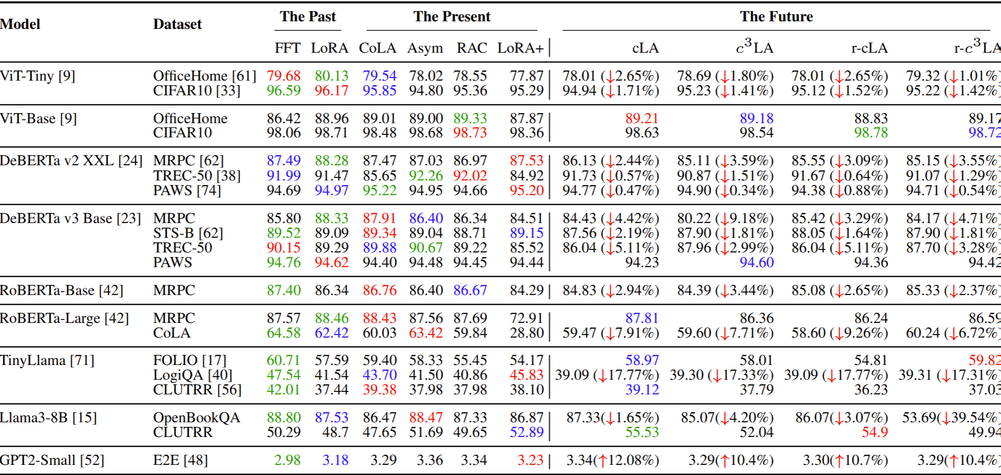
The full empirical comparison reports performance and generalization over 11 fine-tuning methods. For CoLA we report the Matthews correlation coefficient (higher is better); for GPT2-small, perplexity (lower is better); and for the remaining datasets, accuracy. We use green, red, and blue to indicate the best, second best, and third best result. For the sparse variants, ↓ indicates the accuracy drop percentage compared to the best.

Performance of fine-tuned models across the past, present, and future PEFT methods.

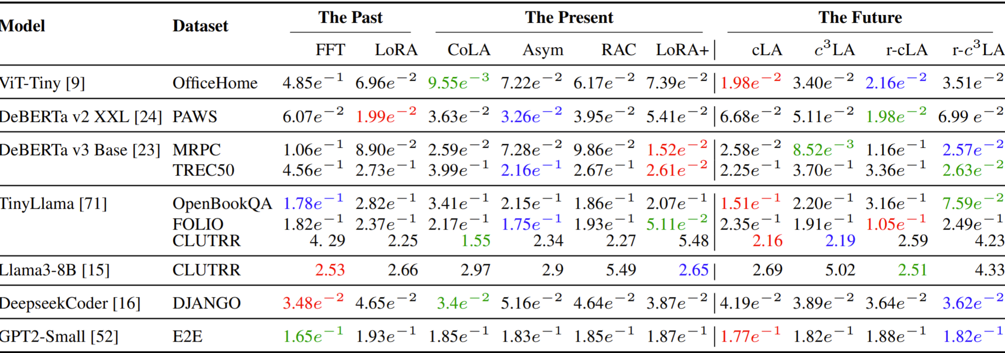
Empirical generalization error, 𝒢(W), of the fine-tuning methods over various models and datasets. Lower values are better. These values are approximations for how far off the loss of the model obtained on the training set will match the loss of the model on its entire input space (thus its loss in training will better match its loss on any sufficiently large dataset observed in a production environment).

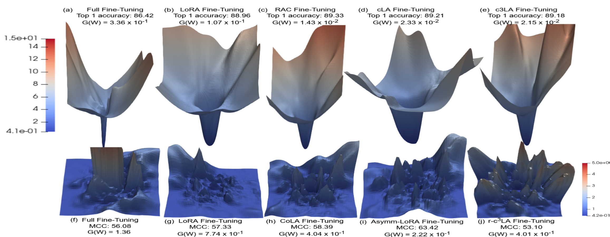
Diagnostics: When Sharpness and Generalization Disagree

Loss landscapes and intruder dimensions are useful diagnostics, but they do not consistently align with empirical generalization error or test performance. Chain variants often produce sharper landscapes and more intruder dimensions than their non-chain counterparts, but this does not necessarily imply worse empirical generalization.

The key takeaway is that these diagnostics can provide useful post hoc explanations, but they can also produce false positives. In this paper, we show that our information-theoretic generalization bounds predict our empirical generalization results (where lower bounds result in lower generalization) more consistently than loss landscapes and intruder dimensions.

Loss landscapes of ViT-Base fined tuned on OfficeHome (top row) with PCA directions, and RoBERTa-Base fine-tuned on CoLA (bottom row) with random directions. Note in (b) and (c) where RAC-LoRA produces a spikier landscape than LoRA while reporting better generalization error empirically. This better generalization is predicted by our information-theoretic bounds (for the chain length we ran in this experiment), as only training the B-matrix reduces the bound.

Closing Takeaways

• PEFT performance is task-dependent: no single fine-tuning method dominates across all models and datasets.
• Our proposed sparse extensions of SOTA LoRA variants perform well across multiple modalities and models while substantially reducing training time and memory requirements
• From a theoretical perspective, our sparsity-induced variants serve as a bridge between LoRA and PaCA, two different families of PEFT methods. While these sparse variants may require larger budgets to maintain robustness in certain settings, they remain overall effective, highlighting the importance of selecting fine- tuning methods based on task characteristics and user constraints
• We show that, in theory, the sparse methods have the same generalization error upper bounds as their non-sparse counterparts, and closely track the empirical generalization trend across most models and modalities. This insight provides a more consistent and guided pathway for selecting PEFT methods, complementing existing diagnostic tools such as loss-landscape and intruder-dimension analyses.

Citation

@article{beyondlora,
  title={Beyond LoRA: Is Sparsity-Induced Adaptation Better?},
  author={Cadenhead, Elijah and McGee, Cristian and Li, Xin and Bergou, El Houcine and Dutta, Aritra},
  year={2026}
}